This workflow will provide an overview of how to use BNW to:

1) Select a structure learning method and upload data into BNW

2) Use the BNW structural restraint interface

3) Make predictions with the network structure

1. Select structure learning method and uploading data into BNW

For this workflow, we are creating a network using a biological data set containing both continuous and discrete variables. The variables are a genotype (the discrete variable), three gene expression traits (Gene1, Gene2, Gene3), and a phenotype.

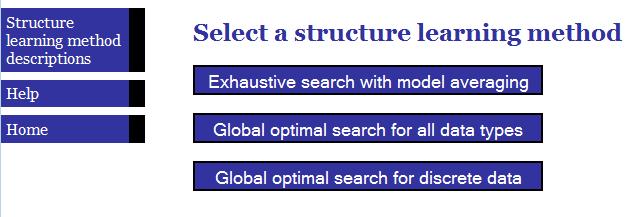
We do not know the network structure for this dataset, so we will first use BNW to learn the structure. Selecting Learn a network model from data on the BNW home page presents a list of the three structure learning methods that are currently implemented in BNW.

Because the network contains only 5 variables, we can use any of these structure learning methods. If more than 6 variables are present, using the global optimal search method would likely be necessary. We will use the exhaustive search with model averaging method in this workflow. More information about the structure learning methods can be found on the BNW help page.

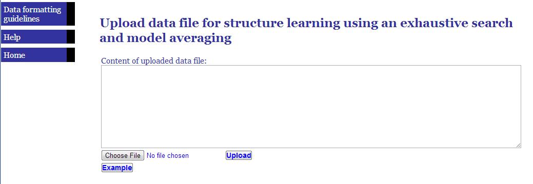
After selecting the Exhaustive Search button, we are prompted to upload a file containing the data.

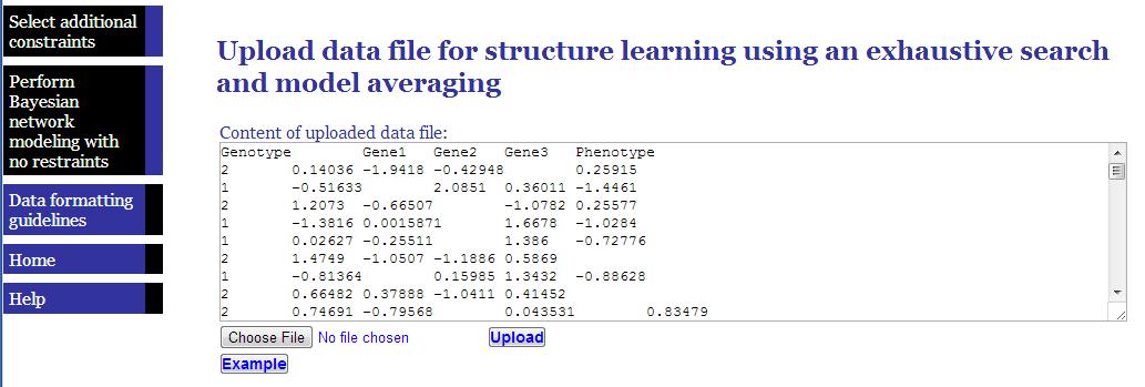
The figure below shows BNW after we have uploaded the data file. The first line of the data contains the names of the variables included in the network, while the remaining lines are the variable values for individual samples. A description of how to format data files for use in BNW can be found on the BNW help page and can be accessed by the the Data formatting guidelines option in the left menu. Additionally, two additional options, Select additional constraints or Perform Bayesian network modeling with no restraints, appear in the left menu after loading the data file.

2. Use the structural constraint interface

Here, we will use the structural constraint interface to help identify biologically meaningful network structures. Specifically, we want to investigate how the genotype impacts gene expression which then impacts the phenotype.

The first section of the structural constraint interface allows users to assign the variables (nodes) in the network to tiers. By default, three tiers are shown, but this can be changed by selecting a different number in the drop-down menu. The leftmost box of this section contains draggable boxes with the names of the variables in the network.

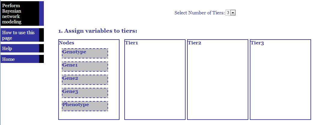
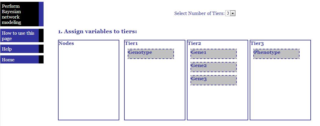
For this network, we want to assign Genotype to Tier1, the gene expression traits to Tier2, and the Phenotype to Tier3.

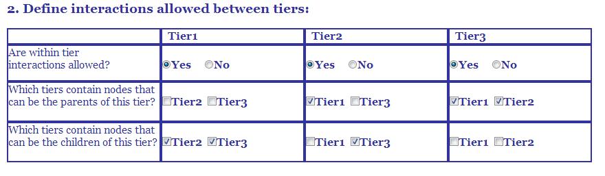
The second section in the structural constraint interface allows users to specify the types of interactions that are allowed both between and within tiers. In this case, we will keep the default settings, which will allow there to be edges between nodes within a tier, prevent nodes in Tier1 from being the child of Tier2 and Tier3 nodes, and prevent nodes in Tier2 from being the child of Tier2 nodes.

The final section of the structural constraint interface would allow for the specification of particular edges that should be banned from the network or required to be in the network. Users can identify these edges by dragging the nodes to appropriate boxes. In this case, we do not want to ban or require any specific edges.

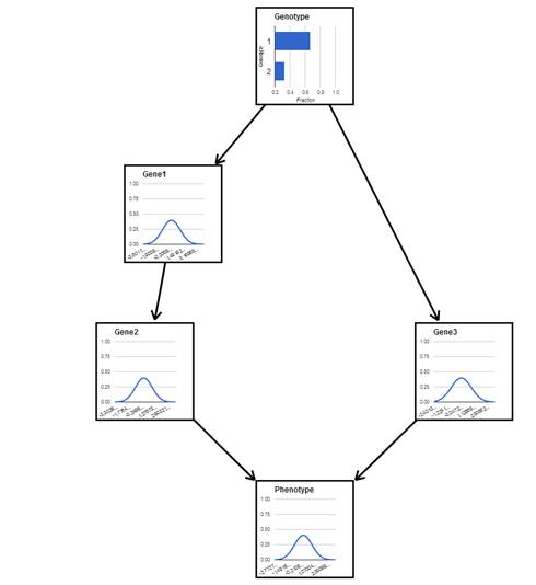
After entering the structural constraints, BNW will perform structure learning from the data after clicking Perform Bayesin network modeling on the left menu and present the structure of the network as shown below. Genotype, the discrete node, is shown as a bar chart with the bars showing the fraction of samples with each genotype in the data, while the other nodes are shown as lines with the Gaussian distributions that best fit the data.

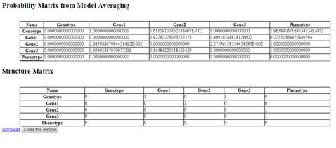
To further investigate the structure of the network, users can select Display Structure Matrix in the left menu. This will bring up a popup windoe containing a table showing the confidence of each directed edge in the network after model averaging. For this network, all of the nodes included in the network were present in almost all high scoring networks, as the values of the edges are all near 1. BNW displays all edges with a confidence greater than 0.5 in the network structure. A second table in the window shows the structure matrix with a 1 for edges included in the structure and 0 for edges that are not included. These tables can be downloaded by clicking the download link.

3) Make predictions with the network structure

BNW can be used to both predict the values of variables in a network given known evidence and to investigate how the network might change in response to interventions. Users can switch between evidence and intervention modes by selecting the proper button on the top of the page containing the network structure.

For example, suppose we want to use the model to make predictions for a new sample that was not in the original dataset. We know that this sample was from an individual with Genotype=2 and want to predict the values of the genes and phenotype for the individual. To enter this evidence in the network, we simply click on the Genotype node in the network and enter 2 in the popup window.

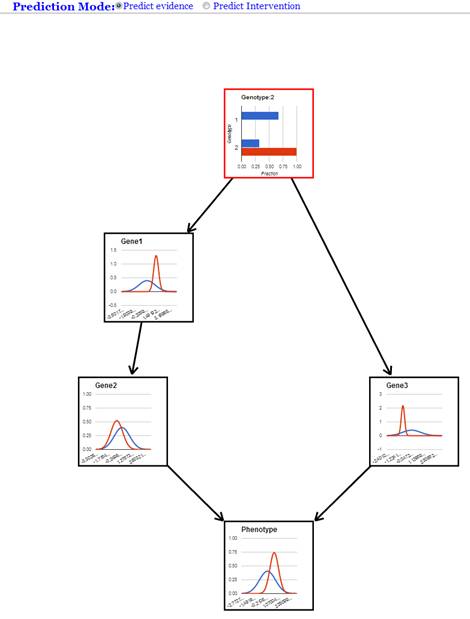
The figure below shows the changes in the network after entering this evidence.The node for which evidence was entered now contains a red outline and all of the nodes in the network now contain both blue and red lines. The blue lines show the original values of the distributions, while the red lines shown the predicted values given the evidence. In this case, knowing that the individual had Genotype=2 would cause us to predict that the expression of Gene1 and the value of the phenotype would be above average, while the expression of Gene2 and Gene3 would be decreases. The specific changes in the predicted values can be investigated by hovering over the nodes and observing the values at the peaks of the distribution.

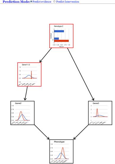
Evidence can be entered in more than one node in the network. For example, the figure below shows predicted values for the network after entering evidence for both Genotype and Gene1.

To use the network to predict the results of intervention, select the proper button on the top of the window to enter intervention mode. While evidence simply changes the predicted values of the other nodes in the network, intervention has a larger effect, as it removes the dependence of the intervened network on its parents and changes the network structure.

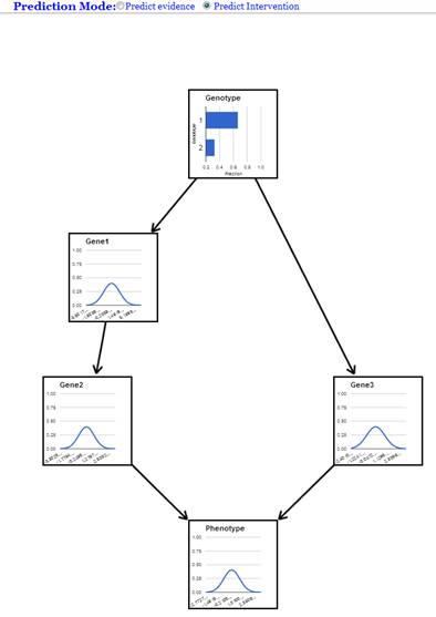
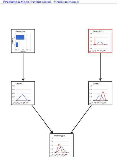
The figure below shows the changes in the network in BNW after intervention on Gene1 that results Gene1 having a low value. The predictions of the network after this intervention could be compared with experiments that prevent Gene1 from being expressed. Intervention that decreases Gene1 is predicted to result in an increase in Gene2 and a decrease in the phenotype. Note that Genotype and Gene3, which are not descendents of Gene1, are not affected by the intervention.